Machine Learning for Drug Discovery in a Nutshell

- by Stefan Schroedl, Head of Machine Learning at Atomwise

Originally posted on Medium

Introduction

Having applied machine learning to search and advertising for many years, two years ago I was ready for a transition to something new. In particular, the field of life sciences seemed to stand out as an opportunity to have a rewarding and positive impact. I was excited to join Atomwise, working on deep learning for drug discovery.

Deep neural networks started to become particularly popular around 2012, when researchers from the University of Toronto [Krizhevsky et al, 2012] won the ImageNet Large Scale Visual Recognition Challenge (ILSVRC). In recent years, this brand of machine learning techniques has revolutionized several artificial fields such as computer vision, natural language processing, and game playing. Will it be able to similarly transform chemistry, biology, and medicine? Experimental sciences give rise to a wealth of unstructured, noisy, and sometimes poorly understood data. One central attraction of deep neural nets is their ability to build complex and suitable featurizations without the need to handcraft them explicitly. Progress has undoubtedly been made, and compelling ideas have been proposed and are being developed. In the same year of the first ImageNet competition, Kaggle hosted the Merck Molecular Activity Challenge; this sparked a lot of interest as well, spurred research into life sciences applications and also captured attention in the popular press. But despite significant progress, it is fair to say that many obstacles and challenges are still waiting to be conquered before an overall breakthrough for practical applications can be declared.

If you are like me, coming from a machine learning or software engineering background but without extensive exposure to medicine, biology, or chemistry, be encouraged: The algorithmic problem can often be formulated and separated cleanly from the (wet) hardware. With this blog post, I am going to try to give you a flavor of and a starting point into the wondrous and peculiar world of drug discovery. It is mainly based on osmosis from my brilliant co-workers, many papers I read and Khan Academy and Youtube videos I watched. There are plenty of excellent online resources available, but be warned: It is really easy to get too deep down into the rabbit hole. I hope this post will help you with some high-level orientation. Needless to say, while trying to cover the breadth fairly, it will be necessarily subjective. Familiarity with machine learning, particularly contemporary neural network approaches, is assumed; it will rather focus on things that seem new and unusual from this perspective. In addition, I would also highly recommend this blog post, as it was quite a helpful introduction to me.

People say the practice of machine learning is (at least) 80% data processing and cleaning and 20% algorithms. This is not different for machine learning in chemistry and biology. I will have to briefly start with the underlying physical sciences and experimentation; touch on cheminformatics representations; and then see how the type of machine learning follows from the structure of the inputs and targets.

This post is organized in two parts (apologies, it grew longer than I originally planned …). This first one will recap the basics of drug mechanisms, the research pipeline, experimental databases, and evaluation metrics. This will set the stage for the second part, in which we delve into greater detail of representation formalisms as well as the range of traditional machine learning and deep learning approaches.

To skip to the conclusion, I found the transition into this field very rewarding. There are plenty of novel, cutting-edge problems that can be addressed by computer scientists and machine learning engineers even without a deep background in life sciences. So if you are curious and interested in getting involved, don’t hesitate!

So now, without further ado, let’s dive right in and recap the basic premises.

How Drugs Work: “Mechanism of Action”

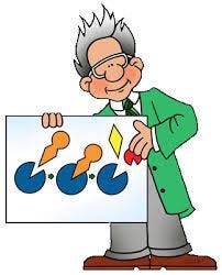
Many proteins in our body are enzymes, which means that they speed up the rate of a chemical reaction without being irreversibly changed themselves. Others are part of signaling pathways that control highly specific cell adaptations and reactions. We can imagine these proteins working via a lock-and-key principle: One or multiple smaller molecules (substrates, ligands) fit snugly into a “hole” (binding pocket, active site) of a protein, thereby facilitating a subtle structure change, which in turn can lead to a domino chain of reactions. Agonists (resp. antagonists) tend to speed up (resp. slow down or block) reactions. Because proteins ‘receive’ signals via other molecules, they are also called receptors. There are also more subtle ways to interact than this competitive inhibition; for example, in allosteric regulation, compounds bind in other places away from the active site, but indirectly affect the reaction through distant conformation changes in the protein.

Binding drug molecules (compounds) are made to be structurally similar to native ligands (the “original” keys); they bind, but fail to induce a reaction and block it by displacing the latter. They are like a fake duplicate key, close enough to fit into the hole, but not of the right shape to turn the lock.

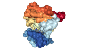These are of course crude simplifications. In practice, proteins and molecules are always in motion, constantly bouncing and wiggling around— there is no clear static binding pose. Often other small molecules such as co-factors or vitamins are involved in the reaction. And a major issue in modeling docking is how to model the interaction with water molecules. As bland as it may seem, water is one of the most difficult things to model! Chemical groups or molecules can be hydrophobic (apolar, water repelling). Water molecules around the surface of the binding pocket and the ligand have to organize in specific patterns; therefore, binding reduces this combined surface and hence increases water entropy.

Most current drugs are of this type described above called “small molecules”, on which we will focus here. They usually consist of less than, say, 10–100 atoms — compared to proteins, which are huge (thousands). Apart from that, other classes of medicines exist and are being developed, such as biologic drugs or therapeutic antibodies.

Stages of Drug Development

I am probably not telling you anything new when saying that the drug development cycle is slow and expensive, 15 years and 2.5 billion dollars — yada yada yada. There are many good online resources you can read about it, e.g. here. Just a brief recap, the development stages are [Hughes et al, 2011]:

• Target selection and validation. Historically pharmaceutical research started from (often serendipitously) observed medical effects. The new paradigm of “rational drug design” turned this on its head, by analyzing biological pathways and thereby identifying “druggable” targets.
• Hit discovery. Screen millions of library compounds, as many and as diverse as possible, to uncover novel activities (side note: millions of compounds sounds a lot, but this is actually a tiny tiny fraction of the chemical universe of drug-like synthesizable compounds, estimated to be around 10⁶⁰.) High throughput screening (HTS) heavily relies on laboratory automation and robotics. In analogy to that, virtual high throughput screening (VHTS) aims at a similar screening procedure but using software only (hopefully faster, cheaper, and more diverse).
• Hit to lead. Limited optimization of promising hits to increase affinity. Because (V)HTS data is huge but of low accuracy, any potential hits has to be confirmed, ideally using multiple independent types of assays.
• Lead optimization. Further directed optimization to generate viable drug candidates. Note that target affinity is only one of several factors that decide if a compound can become a practically viable medicine. Other factors are pharmacodynamics (biochemical and physical effects of drugs on the living organism) and pharmacokinetics (how the living organism acts on the drug). You might also see the acronym ADMET: absorption, distribution, metabolism, and excretion, toxicity. Note that toxicity means that the drug binds to targets other than the intended ones, i.e., low selectivity.
• Pre-clinical development. In-vitro, in-situ, in-vivo, and animal testing.
• No matter how amazing ML techniques can be, they will never replace clinical trials. Predominantly 3 phases with successively larger groups of patients, to ensure safety and effectiveness.

Clinical trials are the precondition for FDA approval. An interesting tidbit is the fact that the total number of approved drugs is currently around 1500 — much lower than I would have guessed. And the distribution of drug targets is highly skewed: Around 40% of all medicinal drugs target just one superfamily of receptors — the G-protein coupled receptors (GPCRs), signaling proteins anchored in the cell wall. Another prominent class are kinases, which act by attaching phosphor groups to other proteins.

In this post, I will focus on the use of machine learning in the context of VHTS and hit-to-lead/lead optimization (in the latter case, the technical term is QSAR — quantitative structure activity relationship, i.e., models to predict binding affinity values from compound and possibly protein features). A few larger companies (e.g., IBM Watson) and startups also work on supporting target selection, e.g., by mining vast amounts of clinical, genomic, expression, and text data from publications. However, here I will not discuss these approaches further.

What initially confused me was that researchers make fine grained distinction between hit discovery/hit-to-lead and lead optimization. From a purely machine learning standpoint, you would expected the goal and methods to be identical: find a compound with a high binding affinity (and maybe, as a bonus, good metabolic properties). Even so-called “docking” methods to identify the spatial protein-ligand interaction could be seen as one approach to it; but as we will see later, it is treated as its own separate category of algorithms.

The varying degrees of a) noise in the data and b) computational budget due to the size and success rate of the candidate set, give rise to different approaches. ML for VHTS must be fast, have good ranking performance, while precision of score values matters. On the other hand, QSAR applications can be more elaborate, don’t need to deal too well with non-binders, but should predict binding affinity with high accuracy and correlation.

Data and Assays

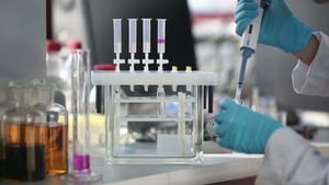When medicinal chemists use the term assay, they might refer to a plethora of experimental measurement types: From chemical concentrations or reaction rates, to observations in single cells tissues, or even whole animal models. biological drug activity (a.k.a. affinity, potency) is usually expressed as a concentration necessary to induce some observation, e.g., to reduce a chemical rate of an enzyme reaction by 50% (this is called IC50). Individual high-throughput assays are typically run at a single fixed concentration. A more granular dose-response curve (and associated IC50) can be estimated from fitting a curve to 4 or more experimental points. These measurements are inherently very noisy, since they depend on a host of environmental influences; in addition to acting on the target, compounds can also interfere in various ways with the mechanism of observation, e.g., luminescence. Running the same binding assay twice in the same pharmaceutical lab has been estimated to have an average 2–3 fold uncertainty; the variation can easily be a factor of 5–10 for different labs (this has also been roughly estimated from publicly available data on repeated measurements [Kramer et al, 2012]). This is what chemists call “about the same”! Due to the large dynamic range of measurements, affinities are mostly specified on a negative logarithmic scale (an IC50 of, say, 10 micromols corresponds to a pIC50 of 5 — note that smaller concentrations, but larger pIC50 are more potent). The hit-to-lead phase is usually expected to yield compounds within a potency range of 5–7.

We could see it as a “chemical version of the uncertainty principle”: with increasing complexity of experiments, from pure binding assays to multi-step chemical reactions to cell- and animal-based assays, biological relevance increases with respect to the ultimate goal of developing a viable medicine; but so does the measurement noise as well. Even simple molecular properties can only be known to a limited precision; this unavoidable label noise is referred to as chemical accuracy.

In addition to experimentation error, the medical and biochemical literature is heavily subject to publication bias. Incentives exists to report positive results, but naturally less so for negative results or repetition of previous experiments. In fact, the entire drug discovery pipeline is usually geared towards “failing fast and cheap”, i.e., eliminating unpromising candidates as early as possible (no point in spending money to find out how inactive exactly an inactive compound is). Consequently, negative data is scarce and has low accuracy.

Chembl is a public database containing millions of bioactive molecules and assay results. The data has been manually transcribed and curated from publications. Chembl is an invaluable source, but it is not without errors — e.g., sometimes affinities are off by exactly 3 or 6 orders of magnitude due to wrongly transcribed units (micromols instead of nanomols).

Patents come with their own particular issues. Obviously, they are under the incentive to be as broad as possible. So they often contain tables with one column for a molecule diagram, and another column for the associated affinity value. But the molecule can contain one or multiple R-groups, where R can be substituted by multiple groups as listed in the text. Obviously, not all these (sometimes hundreds of) molecules can have exactly the same affinity. On average, affinities from patents are higher than those from publications, since the pharmaceutical industry strives to optimize ligand potency as much as possible, while academic research is more focused on basic research and early stage candidates.

Pharmaceutical companies maintain their own proprietary databases of experimental results, and assemble large libraries of molecules that are routinely used in screening. The scale and reproducibility of internal databases exceeds all publicly available data probably by an order of magnitude.

Benchmarks

In the image recognition domain, very large benchmark datasets (e.g., ImageNet) exist and researchers can more or less agree on uncontroversial evaluation criteria. This allows the predictive accuracy of different techniques to be be adequately quantified and compared. Unfortunately, this is currently not the case for virtual screening and QSAR; indeed, machine learning in drug discovery has been held back by the lack of such common standards and metrics.

It is not that efforts in this direction wouldn’t have been undertaken. The widely used DUDE-E benchmark [Mysinger et al, 2014] chose challenging decoys (negative examples) by making them similar to binders (positive examples) in terms of 1-D properties such as molecular weight, rotatable bonds, etc, but at the same time be topologically dissimilar to minimize the likelihood of actual binding. For the ‘topologically dissimilar’ part, 2-D fingerprints were used. Later it was convenient for researchers to continue to publish their method’s accuracy in terms of this benchmark, even for QSAR methods for which DUD-E had not been designed. Not too surprisingly then, fingerprint-based methods turned out to excel at this task — and hence justified the publications.

Another frequently used database is PDBbind, which contains protein-ligand co-crystal structures together with binding affinity values. Again, while certainly very valuable, PDBbind has some well-known data problems. Most authors have adhered to a data split with significant overlap or similarity between examples in the train and test sets. Some works have not distinguished between validation and test. Though there have been updated versions over the years, the 2007 version is still frequently used in order to maintain comparability with previous publications.

More broadly, the question of how to split existing data into training and test is actually quite tricky — I can attest to the fact that by choosing a particular such scheme, almost any model can be made look excellent or mediocre!

Classical machine learning literature spends little attention to this aspect. Most often, the underlying assumption is that training and test examples are drawn i.i.d. from the same distribution. However, this does not necessarily reflect a good indicator of prospective performance in drug discovery. A random split is usually overly optimistic, since molecules and targets can be the same or very similar between training and test. Sometimes, when chemists plan which molecules to synthesize next, they intentionally choose ones that are dissimilar from those they already know, in order to explore a larger chemical space. One sensible approach is time split, simulating the inference of future data at a particular moment. Alternatively, [Martin et al, 2017] cluster the compounds for a given target, and sort the smallest cluster to the test set. We see that the topic of bias in drug discovery datasets is a thorny one [Wallach and Heifets, 2018] …

We have mentioned above that negative examples (in this context sometimes called decoys) are hard to retrieve from publicly available sources; and those that do exist have noisier measurements, they might in fact be false negatives. The way we choose negative examples exerts a strong influence on our models and outcomes. We could make the simplifying assumption that since biological activity is a rare phenomenon, any molecule is presumed inactive until proved otherwise. Then, we could proceed with an approach like PU-learning (only positives and unknown labels are given, see e.g., [Han et al 2016]), or we could generate synthetic examples. But the prediction model will still be influenced by the chosen sampling distribution. And for QSAR, it is even harder to invent not only the class (positive/negative), but also an actual affinity value as target.

Metrics

Let us now turn to the question of how to choose appropriate evaluation criteria. A good metric should be [Lopes et al, 2017]: sensitive to algorithm variations, but insensitive of data set properties; statistically robust; have as few parameters as possible; have straightforward error bounds; have a common range of values, regardless of data; and be easily understandable and interpretable.

In lead optimization, we want to obtain precise, continuous binding affinity predictions for not too many different compounds, so a standard metrics would be root mean square error. Measures intended to reduce the influence of outliers, such as mean absolute error or Huber loss, are reasonable choices as well.

The situation can be much tougher in virtual high throughput screening. Let’s work backward from the ultimate use case: Assume we have a set of 100,000 potential candidate molecules, out of which 500 are true hits. We run our latest newfangled model and rank all candidates by score. Now we can select the top 1000 molecules and use a chemical assay to try to confirm our model’s prediction. By chance, we would expect to find 5 hits. If the tests now reveal, say, 20 hits in the list of top-ranked candidates, we would say our model has an enrichment factor of 4 (funny how this metric sounds like something chemical itself?).

While the enrichment factor metric is intuitive and well understood by chemists, it is however not great to operate with: it strongly depends on the ratio of positives, on the cutoff, and can saturate. It is also hard to convert it into something differentiable to use for gradient descent.

A host of other metrics has been proposed in the literature. The area under the ROC curve (AUC) is widely used in other domains as well; it is independent of the positive rate and has an intuitive probabilistic interpretation. Its drawback is that it is a classification measure — instead, we should give more weight to the early positions in the ranking. The (ranked) correlation coefficient implicitly assumes a linear relationship. Another measure, the area under the accumulation curve (AUAC), was shown to be functionally related to AUC, and to the average rank of positives, as well. Validated by simulations, the power metrics [Lopes et al, 2017], defined as TPR/(TPR+FPR)), was proposed as an improvement. Robust initial enrichment (RIE) is parameterized by an exponential weighting of the ranks of positives, as an alternative to a hard cutoff; BEDROC [Truchon and Bayly, 2007] is derived from RIE by normalizing the range of possible values to [0,1]. Unfortunately, a drawback by many of these metrics not shared by AUC is that they depend on the overall positive rate, which is not related to algorithm performance.

An eye-opening paper on the pitfalls of benchmarks and metrics is [Gabel et al, 2014]. A random forest model was trained on PDBbind for affinity prediction from co-crystals; the features were distance-binned counts of protein-ligand atom pairs. This model strongly outperforms a standard force-field based scoring function on this dataset. But surprisingly, when applying the same model for the task of finding the right poses (relative positions between ligands and proteins), or on the DUD-E dataset for virtual screening, the model performs rather poorly. Through a number of ablation experiments, the authors show that the learned score in fact relies on type atom counts, and is almost independent of protein-ligand interactions.

While there is a lot more material that we could get into, I will stop at this point but hope that I could give you a brief glimpse of the drug discovery problem, its data sets, benchmarks, and evaluation metrics. In the next installment, we will dive into more details of concrete machine learning approaches.

References

• Axen, S. D., Huang, X. P., Cáceres, E. L., Gendelev, L., Roth, B. L., & Keiser, M. J. (2017). A Simple Representation of Three-Dimensional Molecular Structure. Journal of Medicinal Chemistry, 60(17), 7393–7409. https://doi.org/10.1021/acs.jmedchem.7b00696
• Ballester, P. J., & Mitchell, J. B. O. (2010). A machine learning approach to predicting protein-ligand binding affinity with applications to molecular docking. Bioinformatics (Oxford, England), 26(9), 1169–75. https://doi.org/10.1093/bioinformatics/btq112
• Cramer, R. D., Patterson, D. E., & Bunce, J. D. (1988). Comparative Molecular Field Analysis (CoMFA). 1. Effect of Shape on Binding of Steroids to Carrier Proteins. Journal of the American Chemical Society, 110(18), 5959–5967. https://doi.org/10.1021/ja00226a005
• Da, C., & Kireev, D. (2014). Structural protein-ligand interaction fingerprints (SPLIF) for structure-based virtual screening: Method and benchmark study. Journal of Chemical Information and Modeling, 54(9), 2555–2561. https://doi.org/10.1021/ci500319f
• Dahl, G. E., Jaitly, N., & Salakhutdinov, R. (2014). Multi-task Neural Networks for QSAR Predictions. Retrieved from https://arxiv.org/pdf/1406.1231.pdf
• Dieleman, S., De Fauw, J., & Kavukcuoglu, K. (2016). Exploiting Cyclic Symmetry in Convolutional Neural Networks. Retrieved from http://arxiv.org/abs/1602.02660
• Dietterich, T. G., Lathrop, R. H., & Lozano-Pérez, T. (1997). Solving the multiple instance problem with axis-parallel rectangles. Artificial Intelligence, 89(1–2), 31–71. https://doi.org/10.1016/S0004-3702(96)00034-3
• Duvenaud, D., Maclaurin, D., Aguilera-Iparraguirre, J., Gómez-Bombarelli, R., Hirzel, T., Aspuru-Guzik, A., & Adams, R. P. (2015). Convolutional Networks on Graphs for Learning Molecular Fingerprints. Neural Information Processing, 1–9. http://arxiv.org/abs/1509.09292
• Faber, F. A., Hutchison, L., Huang, B., Gilmer, J., Schoenholz, S. S., Dahl, G. E., … von Lilienfeld, O. A. (2017). Machine learning prediction errors better than DFT accuracy, 1–12. Retrieved from http://arxiv.org/abs/1702.05532
• Feinberg, E. N., Sur, D., Husic, B. E., Mai, D., Li, Y., Yang, J., … Pande, V. S. (2018). Spatial Graph Convolutions for Drug Discovery, 1–14. Retrieved from http://arxiv.org/abs/1803.04465
• Gabel, J., Desaphy, J., & Rognan, D. (2014). Beware of machine learning-based scoring functions — On the danger of developing black boxes . Beware of machine learning-based scoring functions — On the danger of developing black boxes. Journal of Chemical Information and Modeling, 54(Ml), 2807–2815. https://doi.org/10.1021/ci500406k
• Gilmer, J., Schoenholz, S. S., Riley, P. F., Vinyals, O., & Dahl, G. E. (2017). Neural Message Passing for Quantum Chemistry. Retrieved from http://arxiv.org/abs/1704.01212
• Gómez-Bombarelli, R., Wei, J. N., Duvenaud, D., Hernández-Lobato, J. M., Sánchez-Lengeling, B., Sheberla, D., … Aspuru-Guzik, A. (2016). Automatic chemical design using a data-driven continuous representation of molecules. ACS Central Science, 4(2), 268–276. https://doi.org/10.1021/acscentsci.7b00572
• Han, J., Zuo, W., Liu, L., Xu, Y., & Peng, T. (2016). Building text classifiers using positive, unlabeled and ‘outdated’ examples. Concurrency Computation, 28(13), 3691–3706. https://doi.org/10.1002/cpe.3879
• Hughes, J. P., Rees, S., Kalindjian, S. B., & Philpott, K. L. (2011). Principles of early drug discovery. British Journal of Pharmacology, 162(6), 1239–49. https://doi.org/10.1111/j.1476-5381.2010.01127.x
• Kadurin, A., Aliper, A., Kazennov, A., Mamoshina, P., Vanhaelen, Q., Khrabrov, K., & Zhavoronkov, A. (2016). The cornucopia of meaningful leads: Applying deep adversarial autoencoders for new molecule development in oncology. Oncotarget, 8(7), 10883–10890. https://doi.org/10.18632/oncotarget.14073
• Kearnes, S., Goldman, B., & Pande, V. (2016). Modeling Industrial ADMET Data with Multitask Networks. https://doi.org/1606.08793v1.pdf
• Kearnes, S., McCloskey, K., Berndl, M., Pande, V., & Riley, P. (2016). Molecular graph convolutions: moving beyond fingerprints. Journal of Computer-Aided Molecular Design, 30(8), 595–608. https://doi.org/10.1007/s10822-016-9938-8
• Keiser, M. J., Roth, B. L., Armbruster, B. N., Ernsberger, P., Irwin, J. J., & Shoichet, B. K. (2007). Relating protein pharmacology by ligand chemistry. Nature Biotechnology, 25(2), 197–206. https://doi.org/10.1038/nbt1284
• Kramer, C., Kalliokoski, T., Gedeck, P., & Vulpetti, A. (2012). The experimental uncertainty of heterogeneous public K_i data. Journal of Medicinal Chemistry, 55(11), 5165–5173. https://doi.org/10.1021/jm300131x
• Krizhevsky, A., Sutskever, I., & Hinton, G. E. (2012). ImageNet Classification with Deep Convolutional Neural Networks. Advances In Neural Information Processing Systems, 1–9.https://papers.nips.cc/paper/4824-imagenet-classification-with-deep-convolutional-neural-networks
• Lenselink, E. B., Jespers, W., Van Vlijmen, H. W. T. T., IJzerman, A. P., & van Westen, G. J. P. P. (2016). Interacting with GPCRs: Using Interaction Fingerprints for Virtual Screening. Journal of Chemical Information and Modeling, 56(10), 2053–2060. https://doi.org/10.1021/acs.jcim.6b00314
• Lenselink, E. B., Ten Dijke, N., Bongers, B., Papadatos, G., Van Vlijmen, H. W. T., Kowalczyk, W., … Van Westen, G. J. P. (2017). Beyond the hype: deep neural networks outperform established methods using a ChEMBL bioactivity benchmark set. Journal of Cheminformatics, 9(1), 1–14. https://doi.org/10.1186/s13321-017-0232-0
• Li, H., Leung, K. S., Wong, M. H., & Ballester, P. J. (2015). Improving autodock vina using random forest: The growing accuracy of binding affinity prediction by the effective exploitation of larger data sets. Molecular Informatics, 34(2–3), 115–126. https://doi.org/10.1002/minf.201400132
• Li, H., Leung, K. S., Wong, M. H., & Ballester, P. J. (2016). Correcting the impact of docking pose generation error on binding affinity prediction. In BMC bioinformatics (Vol. 8623). https://doi.org/10.1007/978-3-319-24462-4_20
• Li, Y., Han, L., Liu, Z., & Wang, R. (2014). Comparative assessment of scoring functions on an updated benchmark: 2. evaluation methods and general results. Journal of Chemical Information and Modeling, 54(6), 1717–1736. https://doi.org/10.1021/ci500081m
• Lopes, J. C. D., Dos Santos, F. M., Martins-José, A., Augustyns, K., & De Winter, H. (2017). The power metric: A new statistically robust enrichment-type metric for virtual screening applications with early recovery capability. Journal of Cheminformatics, 9(1), 1–11. https://doi.org/10.1186/s13321-016-0189-4
• Martin, E. J., Polyakov, V. R., Tian, L., & Perez, R. C. (2017). Profile-QSAR 2.0: Kinase Virtual Screening Accuracy Comparable to Four-Concentration IC50s for Realistically Novel Compounds. Journal of Chemical Information and Modeling, 57(8), 2077–2088. https://doi.org/10.1021/acs.jcim.7b00166
• Mysinger, M. M., Carchia, M., Irwin, J. J., & Shoichet, B. K. (2014). Directory of Useful Decoys, Enhanced (DUD-E): Better Ligands and Decoys for Better Benchmarking. Nucleic Acids Res, 42, 1083–1090.
• Ragoza, M., Turner, L., & Koes, D. R. (2017). Ligand Pose Optimization with Atomic Grid-Based Convolutional Neural Networks. Retrieved from https://arxiv.org/pdf/1710.07400.pdf
• Sanchez-Lengeling, B., Outeiral, C., Guimaraes, G. L., & Aspuru-Guzik, A. (2017). Optimizing distributions over molecular space. An Objective-Reinforced Generative Adversarial Network for Inverse-design Chemistry (ORGANIC). ChemRxiv, 1–18. https://doi.org/10.26434/chemrxiv.5309668.v3
• Smith, J. S., Isayev, O., & Roitberg, A. E. (2017). ANI-1: an extensible neural network potential with DFT accuracy at force field computational cost. Chem. Sci., 8(4), 3192–3203. https://doi.org/10.1039/C6SC05720A
• Thomas, N., Smidt, T., Kearnes, S., Yang, L., Li, L., Kohlhoff, K., & Riley, P. (2018). Tensor Field Networks: Rotation- and Translation-Equivariant Neural Networks for 3D Point Clouds. Retrieved from http://arxiv.org/abs/1802.08219
• Trott, O., & Olson, A. A. J. (2010). AutoDock Vina: improving the speed and accuracy of docking with a new scoring function, efficient optimization and multithreading. Journal of Computational Chemistry, 31(2), 455–461. https://doi.org/10.1002/jcc.21334.AutoDock
• Truchon, J.-F., & Bayly, C. I. (2007). Evaluating Virtual Screening Methods : Good and Bad Metrics for the “ Early Recognition ” Problem Evaluating Virtual Screening Methods : Good and Bad Metrics for the “ Early Recognition ” Problem, 47(February), 488–508. https://doi.org/10.1021/ci600426e
• Wallach, I., Dzamba, M., & Heifets, A. (2015). AtomNet: A Deep Convolutional Neural Network for Bioactivity Prediction in Structure-based Drug Discovery, 1–11. https://doi.org/10.1007/s10618-010-0175-9
• Wallach, I., & Heifets, A. (2018). Most Ligand-Based Classification Benchmarks Reward Memorization Rather than Generalization. Journal of Chemical Information and Modeling, 58(5), 916–932. https://doi.org/10.1021/acs.jcim.7b00403
• Warren, G. L., Andrews, C. V, Capelli, a, Clarke, B., LaLonde, J., Lambert, M. H., … Head, M. S. (2006). A critical assessment of docking programs and scoring functions. Capelli, J. Med. Chem., (49), 5912–5931. https://www.ncbi.nlm.nih.gov/pubmed/17004707
• Xu, Z., Wang, S., Zhu, F., & Huang, J. (2017). Seq2seq fingerprint: An unsupervised deep molecular embedding for drug discovery. … of the 8th ACM International Conference …, 285–294. Retrieved from http://dl.acm.org/citation.cfm?id=3107424